
In a previous blog post, we explored the overall capabilities of ANSYS Simplorer. In this post we will be focusing on Reduced Order Modelling (ROM), specifically the techniques available within Simplorer.
ANSYS has a range of solvers designed to simulate high fidelity models in each of the three main physics areas. When simulating at a System level, most of this detail is not required and could be left out of the overall simulation. For example, a sufficiently detailed model of an electric motor would only need the input voltage/current and the current speed of the motor as inputs and the torque as outputs. It could also be beneficial to add extra inputs such as temperature but knowing the current distribution in the windings or the magnetic field within the structure is not necessary. ROM allows the solver to use a simplified set of equations to determine the output(s) of a model given a particular set of inputs.
ROM has strict limitations which must be considered to achieve an accurate result. Usually ROM is only accurate for a subset of the possible inputs. For example, if a ROM which was used to calculate the thrust of a propeller from the speed of a motor, the model would only hold accurate over a certain range of motor speeds. If the tips of the propeller moved fast enough to enter the transonic or supersonic regions, then the pressure wave in front of the propeller would reduce the thrust generated and the ROM would become increasingly inaccurate. Each particular method for generating ROMs has its own limitations and it is important to consider these when choosing a method.
Importing and Generating Reduced Order Models in ANSYS Simplorer
A large number of different types of models can be imported into ANSYS Simplorer from the various ANSYS solvers as well as several third party software packages (MATLAB Simulink, Mathcad). A couple of the most common ones are covered here.
ANSYS Maxwell
ANSYS Maxwell is particularly well integrated into ANSYS Simplorer. Five different options are provided, of which three are particularly useful for systems design. The Transient solver in ANSYS Maxwell can be directly integrated into the ANSYS Simplorer environment. In this configuration, ANSYS Simplorer will search the ANSYS Maxwell project file for Transient setups and setup a co-simulation link. The time steps between the two solvers are synchronised and the full 3D electromagnetic model is solved. This give the maximum detail but does not generate a ROM.
For models which have behaviour dependent on frequency (such as transformers or multi-conductor cables), ANSYS Simplorer has an option to import a State Space model. First the model is setup in ANSYS Maxwell and a frequency sweep configured. This sweep is then solved once. ANSYS Simplorer can then open the ANSYS Maxwell project and extract a state-space model of the design. This process is automatic with no extra input required.
For models which have behaviour dependent on motion or other geometric changes, ANSYS Simplorer has an option to import an Equivalent Circuit model. First the model is setup in ANSYS Maxwell and a parametric sweep configured. This parametric sweep is then solved. ANSYS Simplorer can then open the ANSYS Maxwell project and extract an equivalent circuit model of the design.
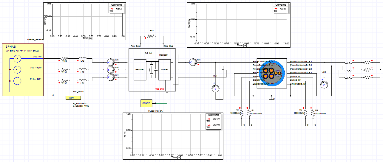
High Power AC Motor System which includes the effect of a long cable run from the drive circuitry to the actual motor. Image Courtesy of ANSYS
ANSYS HFSS and ANSYS SIwave
Although predominantly part of the high frequency domain products, both ANSYS HFSS and ANSYS SIwave can generate ROMs to be used by ANSYS Simplorer. There are two main applications, simulating geometry in order to include parasitics into the design, and allowing waveforms to be pushed from ANSYS Simplorer to ANSYS HFSS/SIwave to excite the geometry (e.g. for EMC analysis or other radiation measurements).
The ROM’s generated by ANSYS HFSS and ANSYS SIwave are very similar. S-parameters of the geometry are simulated vs. frequency which is then used in Simplorer to simulate the effects of the component in question. It is then possible to push those waveforms from ANSYS Simplorer and create the necessary plots, such as the far field radiation pattern or the received signal at another port.
ANSYS Mechanical
There are two main applications for system design with ANSYS Mechanical, modal analysis and rigid body dynamics (RBD). Modal analysis is used to extract how a mechanical model will respond to vibration and this spectrum can be extracted and loaded into ANSYS Simplorer. This has particular applications for analysing equipment such as the exact position of a cutting tool in a CNC machine.
RBD is commonly used to simulate the interactions of a mechanical system with moving parts. For example, a petrol engine can be simulated by applying force to each of the pistons and the resulting torque calculated based on the position of the crank shaft. RBD modelling in ANSYS Simplorer uses co-simulation like ANSYS Maxwell does for transient simulations. RBD is simpler than a full mechanical transient so is viable for use in systems modelling.
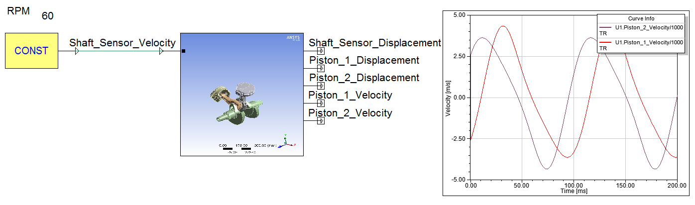
Rigid Body Dynamics Co-simulation in ANSYS Simplorer
ANSYS FLUENT
ANSYS Simplorer supports co-simulation with ANSYS FLUENT in a similar manner to its co-simulation link with ANSYS Maxwell. For most cases however, this is infeasible due to the computation required for transient fluid dynamics simulations. There are two main alternatives which will be covered in greater detail, Linear Time Invariant Reduced Order Modelling (LTI ROM) and Singular Value Decomposition Reduced Order Modelling (SVD-ROM). LTI ROM is available for ANSYS Simplorer 2014 as an extra toolkit and for ANSYS Simplorer 2015 as an integrated component. SVD ROM is still experimental and requires a more manual process as of ANSYS Simplorer 2014.
Linear Time Invariant Reduced Order Modelling
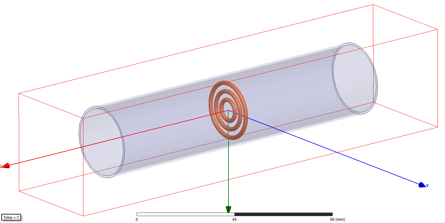
Transient fluid dynamics simulations in particular can take a long time to solve. This makes them impractical for use in a systems design environment. Often only one input variable and one output variable are of interest and yet this requires the entire simulation to be solved. Electronics cooling applications in particular are a prime example of this; the inputs of the model are dissipated power in each component, and the important output is the component and exhaust air temperatures. Consider the following model of a pipe with three circular heating elements.
For this particular example, it can be shown that there is a linear relationship between the dissipated power in each of the heating elements (within reasonable limits) and the temperatures of the components and exhausts. This relationship can be extracted by running a CFD transient with a step response input in power dissipation and then measuring the rise in temperature over time. The steady state result of this is shown below with air flowing from right to left.

LTI ROMs can be very accurate as long as two important limitations are recognised:
- The system must be linear. That is, a five-fold increase in the input must result in a five-fold increase in the output.
- The system must be time-invariant. That is, any propagation delays in the system must stay the same irrespective of the input to the system.
In this example, there is a linear relationship between the power dissipated in the heating elements and the temperature rise at the exhaust. This satisfies the first assumption. Note that this is a valid assumption for reasonable changes in temperature. If the rise in temperature is extreme (say over 500°C or so, the validity of the assumption must be checked before the simulation is relied upon).
The airflow in this example must also be kept constant. If it is varied, then the time delay from the air entering the system to the air leaving the system will change (as well as other boundary wall effects) and the model will be invalid. This is an important limitation to consider when modelling a system.
To generate the final LTI ROM, the CFD simulation is characterised by measuring it’s response to a step input. The LTI toolkit can use an arbitrary number of inputs and outputs but there must be a step response for each combination of inputs and outputs. Based on the step responses loaded, the toolkit then generates a number of transfer functions with increasing order until the model reaches the desired accuracy.
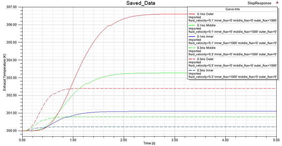
Simulated step response data for each of the three heating elements at two different velocities.
Note that the theory of LTI is not limited to CFD applications. The LTI toolkit can import any data as long as it is formatted correctly and the model will have reasonable accuracy as long as the limitations are accounted for.
Singular Value Decomposition Reduced Order Modelling
LTI ROM is very useful but often the system includes non-time invariant components and the ability to visualise the temperature field within the device would be very useful. Simulating time-variant models is an ongoing research topic but an experimental technique called Singular Value Decomposition Reduced Order Modelling aims to satisfy the second need without resorting to a CFD transient analysis.
SVD is an evolution of LTI, but instead of capturing a single value over time the entire temperature field of the solution is captured. The temperature results can then be loaded into a matrix of size [mesh size, no. of time steps]. So for a simulation with a 106 elements and 200 time steps, the matrix is of size [106, 200]. At this point, it would be possible to create a transfer function relating the temperature of each mesh element to the dissipated power but this would require an impossibly large matrix.
From matrix theory, this matrix can be determined to have a full rank of 200. To perfectly reproduce the results of the CFD analysis, all 200 columns could be used. However it is likely that some of the rows could be added together to create other rows. Consider the matrix below. If the second row is added to the third row, then the result is the first row. Using this method, we could reproduce the original result with only the bottom two rows and an equation for the first row.
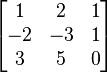
An example of a matrix with a full rank of 3 and a reduced rank of 2 (row rank in this case). Source: http://en.wikipedia.org/wiki/Rank_%28linear_algebra%29
This technique is effective for reducing the memory footprint of the model but the computation required is still very high. With thermal simulations, it is highly likely that a large proportion of the rows will only be loosely related to each other and highly dependent on only a couple of rows. As long as reducing the accuracy of the model slightly is acceptable (this is almost always acceptable with ROM), then the effect of these weak terms could be neglected which would reduce the computation required significantly. With this reduced matrix, we can then generate a state space model and use it to model the CFD solution in ANSYS Simplorer.
Because the relationship between each cell in the matrix is now known, when the simulation in ANSYS Simplorer is complete it is possible to export the results and regenerate the original temperature field in ANSYS FLUENT. This satisfies the limitation of the LTI method which is an in-ability to view the temperature field.
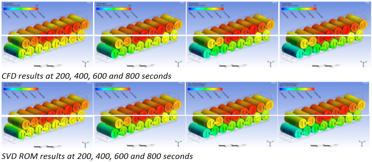
Images and Results Courtesy of ANSYS Inc. and General Motors Company (X. Hu, ”A transient reduced order model for battery thermal management based on singular value decomposition”, IEEE Energy Conversion Congr. and Expo., Pittsburgh, PA, 2014, pp. 3971-3976)
Note that while the LTI toolkit can be used for any time-invariant model in its current state, SVD is limited to use with ANSYS FLUENT at the time of publishing due to the user-defined-functions which are required for generating the results.
Jonathon McMullan
ANSYS Applications Engineer (Electromagnetics and Systems)
jonathon.mcmullan@leapaust.com.au