The world of music is dominated by nonlinear devices. From the wood construction of a guitar neck to the neodymium drivers in PA speakers, every device in the chain has a nonlinear response and these are often exploited to produce a unique sound. To predict with certainty how changes to individual components are going to change the performance of the overall system and therefore the tone generated, we need to consider an entire system.
The Fender Stratocaster is a renowned instrument in the industry densely populated in options. The body, neck, and fretboard are all constructed from different varieties of wood which changes the response and tonality of the guitar body. The construction and materials used in the magnetic pickups also has a major impact on the tonality of the guitar and its useful sustain. Using the ANSYS suite of products, we can break down this system into the key components and analyse each in turn before combining them into a full system. The final audio tracks are embedded here:

Figure 1 – Fender Stratocaster HH, Courtesy of Fender. Image Source: http://www.fender.com.au/products/0149100505.png
Breaking the System Down
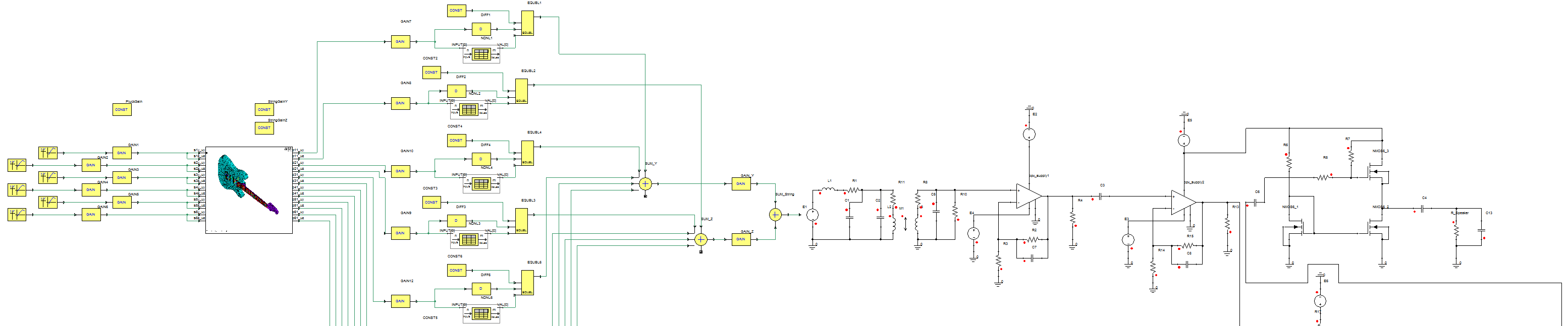
Before we can create suitable simulations for each component, we need to track the relevant signals from inception to the output. In this case the signal is generated by applying a physical force to the string and releasing it quickly. This vibrates the string and the output is a combination of the fundamental frequency of the particular string and a large number of harmonics defined by the construction of the guitar. Some of the vibration is also transferred to the other strings, known as sympathetic ringing.
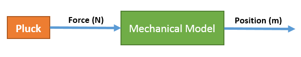
Figure 2 – Calculating the vibration of the string based on the force applied by plucking the string
The motion of the string across the magnetic pickup induces a voltage in the pickup coil. A magnetic pickup is a non-linear device and the non-linear components become more significant as the amplitude of the vibration increases. So the inputs of the magnetic model need to be both the position and the velocity. The velocity is not generated by the Mechanical model but can be derived from the position by taking the derivative.
Figure 3 – Calculating the Output Voltage at the Pickup based on the force applied by plucking the string
From this point forwards, the rest of the system is modelled using an electronic circuit. With the exception of the resistors, all of the components are non-linear with respect to frequency and often with respect to signal amplitude. The combination of all of the models generates the final sound.

Figure 4 – Full System Layout from Input Force to Output Sound
Characterising the Guitar in ANSYS Mechanical
Smoke on the Water by the band Deep Purple has a very distinctive tune which consists of only four notes. To simplify the simulation, we will play single notes rather than chords and the guitar will be open-tuned, i.e. tune each string to play a single note rather than pinching the strings against the fret board.
Here is the geometry of the guitar in ANSYS SpaceClaim. Some of the extraneous features have been removed such as the machine heads to eliminate any geometry which will have minimal impact on the vibration of the strings. The strings have also been simplified to beams using line bodies and assigning a cross-section within SpaceClaim.
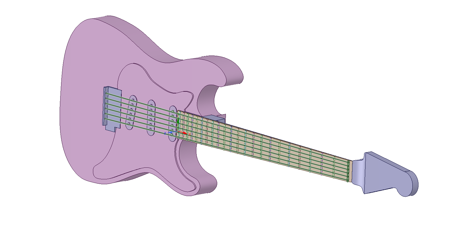
Figure 5 – Simplified Guitar Model in ANSYS SpaceClaim
Simulating the vibration in ANSYS Mechanical requires a two-step analysis. The first step is to pre-tension the strings so that their fundamental frequency is the note which we wish to play. The fundamental frequency of a string is dependent on the length of the string, the tension the string is under, and the distributed mass of the string material.
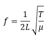
The notes are highlighted in the table below:
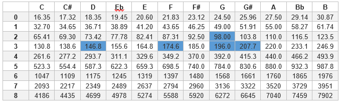
Table 1 – Note frequencies by octave, courtesy of SeventhString. Source: http://www.seventhstring.com/resources/notefrequencies.html
From this information, we can calculate the bolt pretensions required for each string and apply these in a Static Structural analysis. Tensioning each string causes some deflection in the neck of the guitar so some manual tuning will be required after the next step has been completed.

Figure 6 – Deflection of the guitar assembly under pre-tension
This pre-stress loading is then transferred to a Modal analysis to calculate the dominant modes of the entire geometry including the body and neck. After a small modification to the bolt pre-tension to take the deflection of the neck into account, we get the following table of modes:
Table 2 – First 40 calculated modes of the guitar geometry
There are two extra steps required to generate a useful model for importing into ANSYS Simplorer. The first is to add some damping to the model using the MAPDL command “dmprat,0.003”. The second is to calculate the contribution matrix which determines the contribution to the overall amplitude from each mode given an input waveform. A macro is included in the ANSYS installation directory to do this step automatically, ExportStateSpaceMatrices.mac. Remote points are specified on the geometry to specify where the input force is applied and another to specify where the output displacement is calculated. In this example, the top string is plucked at Remote Point input_s1y_uy and the displacement in the string is measured at Remote Point output_p11_uy. Each string has a single input and an output but multiple inputs and outputs are possible for each string if required.
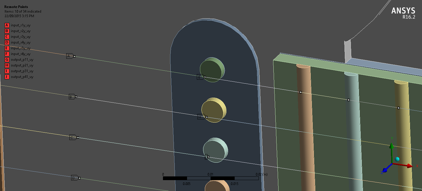
Figure 7 – Remote Points for State Space Model
The macro within Mechanical exports a file with both a pin-configuration and model screenshot ready for importing into Simplorer. After loading and connecting the pluck waveforms to the model, we have the first part of the system.
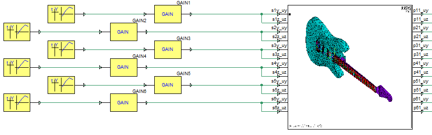
Figure 8 – Mechanical model in a Simplorer Schematic with pluck excitations connected to inputs
Characterising the Magnetic Pickup in ANSYS Maxwell
A magnetic pickup is not a common simulation for ANSYS Maxwell so we will be running a parametric study and characterising the output manually. The pickup has been simplified down to a single pole piece and a short section of the steel string. The fringing effects due to other strings and the other pole pieces are ignored (could be the subject of later investigation). The magnet is comprised of AlNiCo V material and electrical steel has been used for the pole piece (directly below the magnet and wire). The coil has 8000 turns.
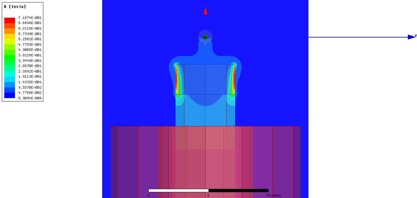
Figure 9 – Magnetic field between the pickup and a stationary string
The magnitude of the voltage induced in the coil is dependent on the velocity of the string passing across the top of the magnet and the strength of the magnetic field at the instantaneous position of the wire. The Transient Solver in ANSYS Maxwell supports translational motion so we can sweep the wire across the top of the pole at a constant velocity and measure the induced voltage in the coil.
To accurately characterise the response of the pickup, we need four relationships. For each axis of motion, we need a relationship between output voltage and velocity in addition to a scale factor depending on the distance between the origin and the string. Eddy currents and magnetic time diffusion are being ignored at present to reduce the mesh density and simulation time. Hence we can assume the trend is linear and this is reflected by simulation.
The major axis with regard to output is the vertical axis. This produces the largest change in magnetic flux through the coil and hence the largest signal output. There is a linear relationship between the velocity and the output signal but a more complex one between the position and output signal. Rather than curve fit the data, the results are loaded into Simplorer directly and interpolated between using the piecewise-linear technique.
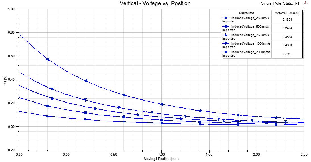
Figure 10 – Plot of output signal for the position sweep along the vertical axis. Multiple velocities are plotted from 250 mm∙s-1 to 2000 mm∙s-1
The horizontal axis is the minor axis. Motion in this direction results in a smaller change in magnetic flux within the coil and hence a smaller output signal. The relationship with velocity remains linear however the relationship between horizontal position and output signal is significantly more complex.

Figure 11 – Plot of output signal for the position sweep along the horizontal axis. Multiple velocities are plotted from 250 mms-1 to 2000 mms-1
The combination of these four equations is what we need to predict this behaviour in ANSYS Simplorer in the final system. Since there is a separate pin for the vertical and horizontal displacements from the Mechanical model, we can isolate the two pickup axes and calculate them in parallel before super imposing the results.
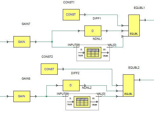
Figure 12 – A single pickup with the major vertical axis and minor horizontal axis modelled independently (inputs at the left, outputs at the right). The equation blocks (EQUBL) are used to scale the result based on the string velocity which is output from the derivative block (DIFF)
Combining the Finite Element models in ANSYS Simplorer with SPICE Modelling
Up until this section, we have focused on modelling the interaction between the player, the guitar and the electronic circuits. ANSYS Simplorer is SPICE compatible so we will be using this technique for modelling the rest of the system. The block diagrams on the left of Figure 1 sum all of the outputs from the pickup models to drive an ideal voltage source. The rest of this circuit models the electrical characteristics of the magnetic pickups and the Direct Input (DI) box which transforms the electrical impedance from 50 kΩ to a 600 Ω XLR connection. All of these resonant circuits emphasize some frequencies and deemphasize others and colour the sound in the process.

Figure 13 – Transferring the output signal from magnetic pickups to the electronic circuits. SUM_String is the total excitation from all five pickups.
For the sake of brevity, the exact function of the rest of the circuit modelling won’t be covered but there is a high resolution screen capture of the entire system is included below. Since the entire system has been modelled, we are able to export the final waveforms to sound files and these are embedded into the webpage. There are two recordings from the output of the circuit, one with a clean output and another with a simple distortion circuit included.
In future we intend to replace the high power amplifiers which drive the speaker and also the distortion pedal with temperature dependent valve models and couple these with CFD to model the transient temperature dependence of the circuit.
The ANSYS Suite of products provides a comprehensive solution for modelling any system and is capable of simulating high fidelity real world products. For further information contact LEAP Australia.
Jonathon McMullan
ANSYS Applications Engineer (Electromagnetics and Systems)