
Today we present a new and easy way to transfer loads from DEM simulations (ROCKY version 3.0 released September 2014) to ANSYS using External Data coupling in ANSYS Workbench.
Discrete Element Method and ROCKY
The Discrete Element Method (DEM) is a computational technique originally developed in the 1970s that has gained great popularity in recent years as advancements in computer hardware technology have allowed much faster and more accurate representations of complex particle systems, as commonly found in bulk materials handling problems. The DEM approach is mainly used for the simulation of granular materials, which consist of a large number of solid particles. DEM can for instance be used to predict and optimize granular flow, belt & liner wear and life, tracking, blockages, spillage, punctures, belt power and capacity.
ROCKY is a powerful and affordable 3D DEM program from Granular Dynamics Inc. (GDI). ROCKY simulates particle behaviour for instance within a conveyor chute, mill, vibrating feeder, crusher, commination machine or any other materials handling system or granular matter.
ROCKY also enables the use of realistically shaped particles in simulations, which provide a more accurate result than using spherical particles. ROCKY can simulate more than 5 million particles with nearly limitless particle shape and size distributions. It also realizes the ability to simulate in different environments, through variable wet, dry, and dust-like conditions. ROCKY’s capabilities include moving boundaries and vibrating surfaces, replicating nearly any type of material and handling environment.
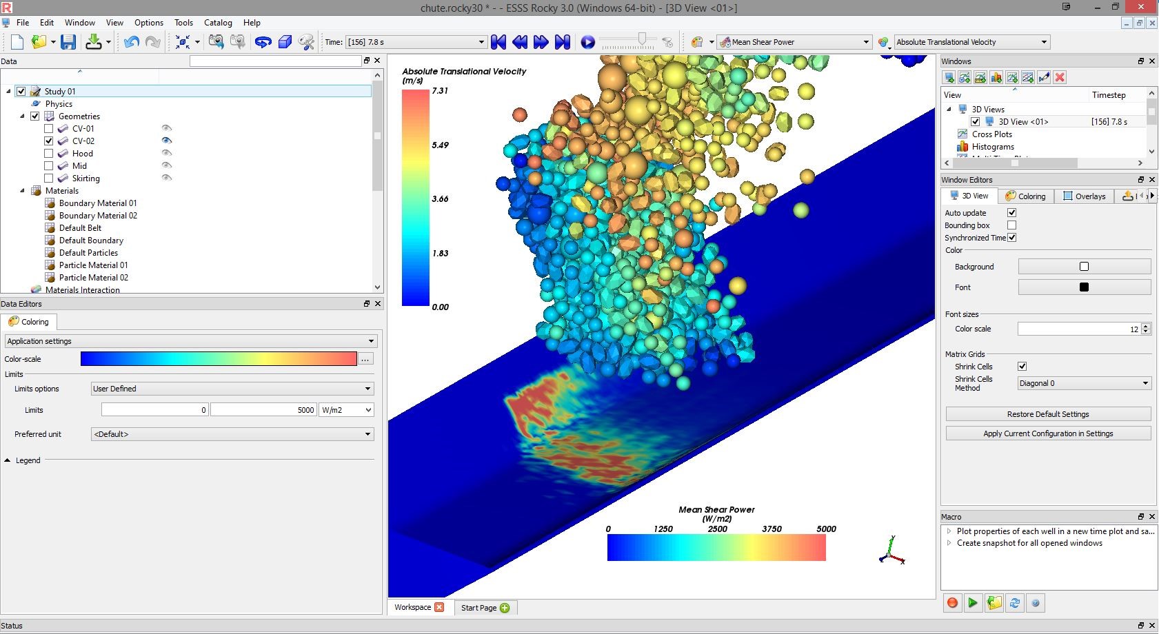
ROCKY 3.0 was released in September 2014 with a completely new user interface, developed in partnership between ESSS and GDI (Granular Dynamics Inc.), along with significant advances in DEM solver technology including the ability to solve using GPU hardware.
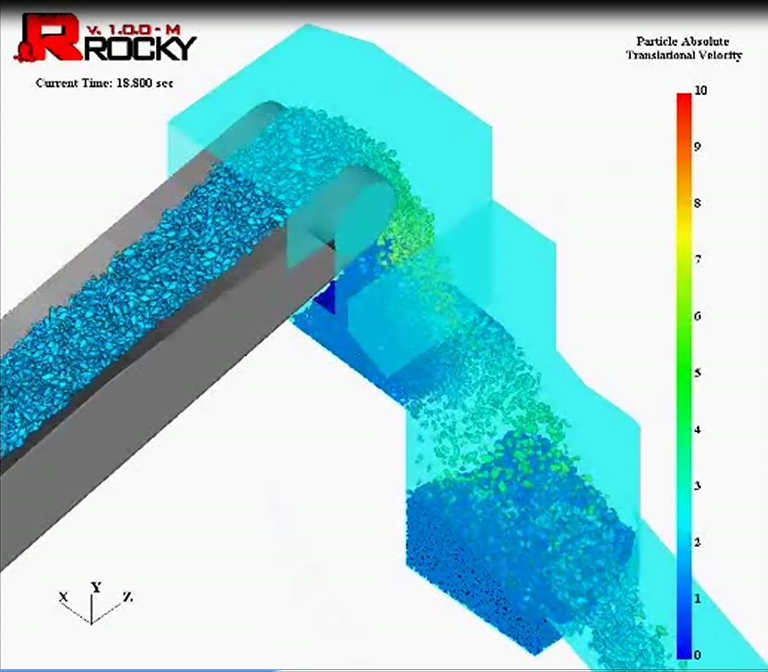
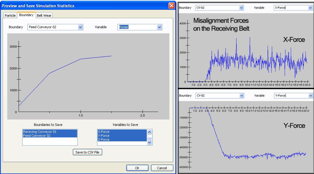
ROCKY examples – mill (top left), chute conveyor (top right) and reaction forces (bottom)

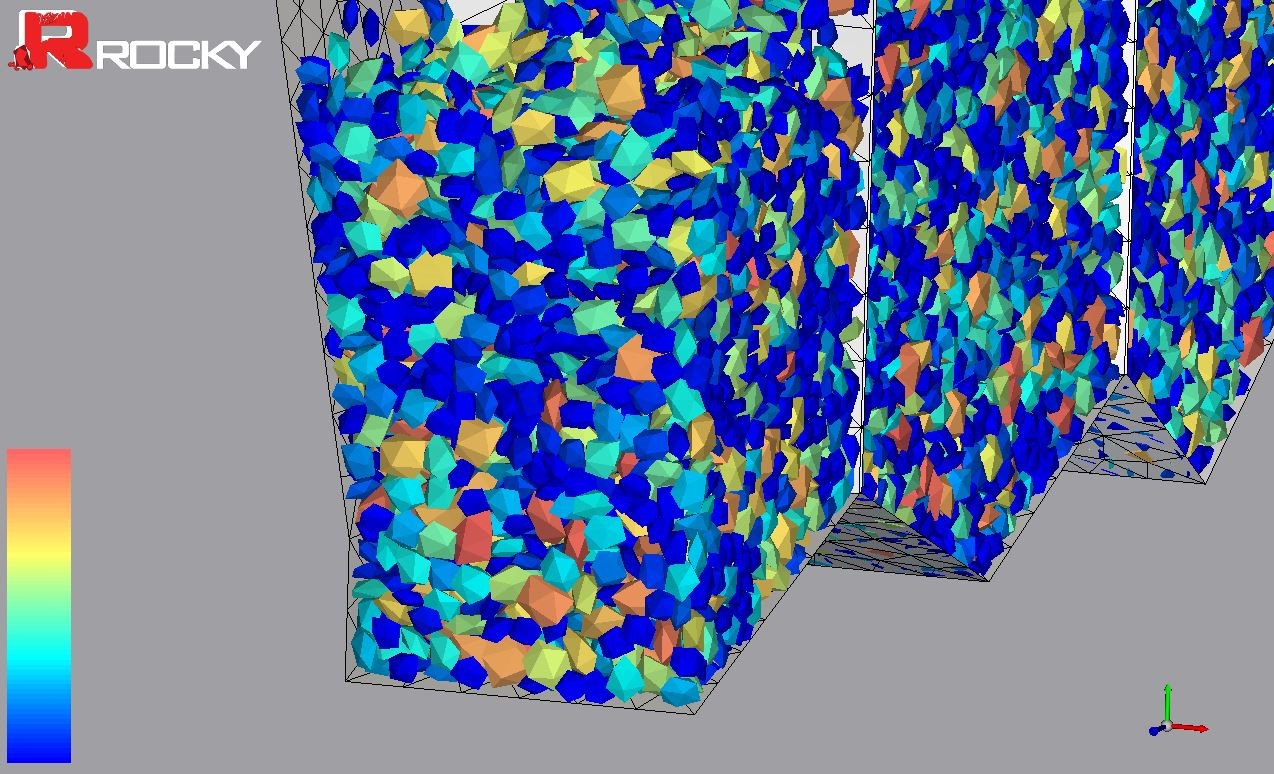
The new ROCKY 3.0 interface showing the particle flow in a hopper
The new ROCKY 3.0 interface showing wear on a belt
ANSYS and Finite Element Analysis (FEA)
Regular readers of our blog will know that FEA tools from ANSYS are used across all engineering disciplines to simulate structural aspects of a product such as stress, deformation, strain and thermal and vibration characteristics.
Transferring loads from ROCKY to ANSYS
Coupling the Discrete Element Method (DEM) of ROCKY with the Finite Element Method (FEM) of ANSYS produces a powerful set of tools capable of predicting not only the flow of particles through bulk materials handling equipment, but also how the particle flow affects the structural integrity of the materials that make up that equipment.
How did you do transfer the ROCKY loads to ANSYS in ROCKY version 2.x?
In older ROCKY versions, two approaches could be used to map the forces from the ROCKY triangular mesh to an ANSYS mesh:
- External DATA approach based on force transfer:
- Does not require a license
- Simple approach
- Limited to (nearly) identical meshes
- The Multifield approach based on force transfer:
- Requires a Mechanical license
- Complicated set-up
- Does not work well for large differences in element size between
ROCKY and ANSYS meshes
Both approaches are based on force transfer, which makes it very difficult to use dissimilar meshes. In reality the ANSYS mesh should often be a lot finer than the ROCKY mesh to predict the stresses in the structure accurately (the ROCKY mesh simply acts as a boundary to the particle flow).
How will you transfer the loads in ROCKY version 3.0?
In ROCKY version 3.0, the nodal area and the pressure components are computed and output directly by ROCKY 3.0. This makes it a lot easier for the user to transfer the loads, as an External Data approach can be used to map the pressures directly to a dissimilar ANSYS mesh. In summary this approach:
– Does not require any additional software license
– Is simple to use and transfers pressures instead of forces
– The ANSYS mesh can be different from the ROCKY mesh
Let’s consider a simple example of how loads are transferred between ROCKY and ANSYS.
Model 1: Bowl Test model
Consider a simple semi-spherical bowl is filled with particles falling through a circular inlet above the bowl, as shown in Figure 1. The inflow is stopped after a certain time to stabilize the particle flow inside the bowl. Table 1 shows the properties of the particles and bowl.
Table 1: Simulation Properties Bowl test Model
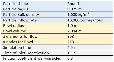
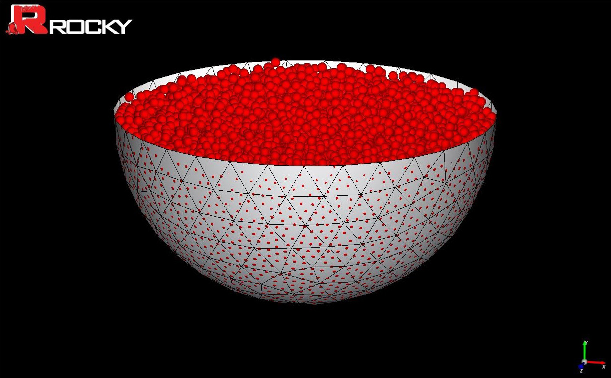
Figure 1: A test model with a bowl of particles used to compute the pressure distribution on the walls
Figure 2 shows the ROCKY vertical reaction force on the bowl versus time. It can be seen that the force has stabilized at the end of the simulation with a final value of 32,088 N. This value is consistent with a simple hand calculation based on the volume of the bowl and the bulk density of the material (assuming the bowl is perfectly filled, which is not exactly the case in the ROCKY model).
F_theoretical=1,600 kg/m3 * 2.094 m3 * 9.8 m/s2= 32,834 N
Preparing the pressure loading for ANSYS is now very easy in ROCKY 3.0:
- Ensure in the ROCKY <Solver – General Settings> tab, the <Collect forces to Fem analysis> is enabled;
- <right click> the bowl body in the <Geometries> tab on the model tree, and select <Export – Ansys Forces>. This will give you a csv file with coordinates, nodal area, forces and pressure components for each node in the model. The coordinates and pressures are used in the ANSYS External Data set-up;
- Your ANSYS mesh can be completely different from your ROCKY mesh, but make sure both meshes are lying in the same spatial x-y-z framework, so that the pressures can be mapped using similar x-y and z locations.
Figure 3 and 4 show the ROCKY normal and tangential stress on the bowl respectively. Figure 5 shows a part of the csv file that is exported from ROCKY.

Figure 2: The ROCKY vertical reaction force on the bowl versus time (final value 32,088 N)
Figure 3: The normal stress in ROCKY displayed in the range 0-25,000 Pa
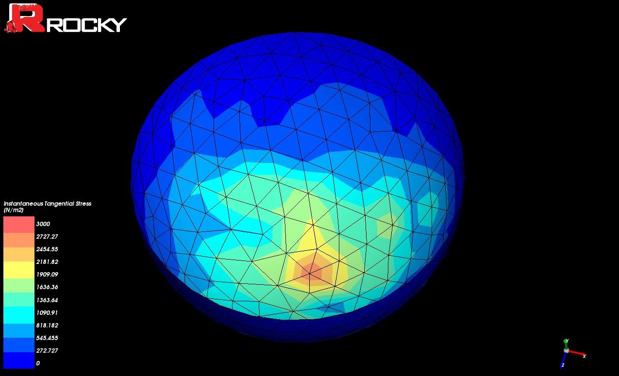
Figure 4: The tangential stress in ROCKY displayed in the range 0-3,000 Pa
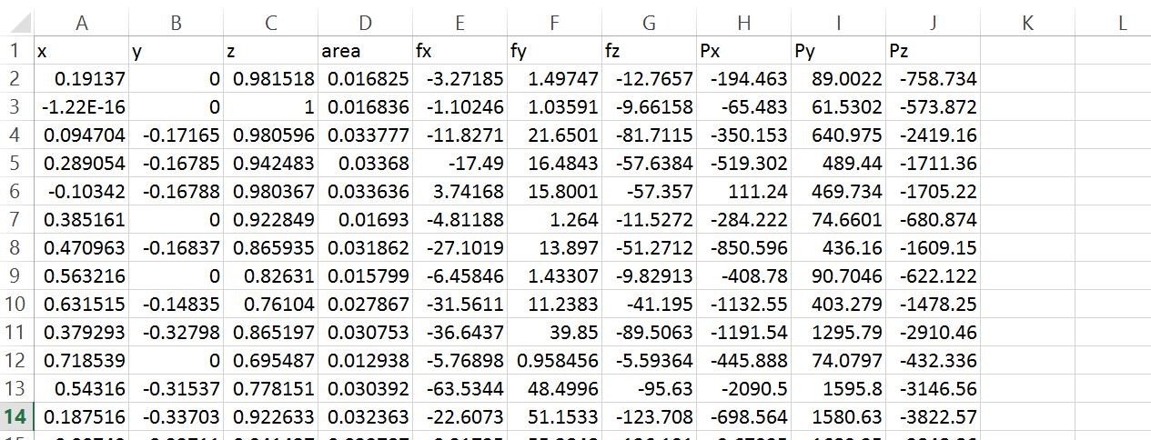
Figure 5: The exported csv file from ROCKY, containing nodal coordinates, nodal area, nodal forces and nodal pressure components
The geometry of the bowl is also prepared for a structural analysis in ANSYS. Both shell elements and solid elements are tested as shown in Figure 6. The mesh is very different from the ROCKY mesh and we have intentionally coarsened one half of the mesh to test the resulting pressure interpolation.
Figure 7 and 8 show how to link the External Data to the model in ANSYS WorkBench. Figure 9 and 10 show the imported pressure in ANSYS Mechanical. Figure 11 shows that the reaction force in ANSYS is similar to the ROCKY reaction force (both for shells and solid shells). Figure 12 shows that the normal stress computed by ANSYS is nearly identical to the normal stress computed by ROCKY.
The bowl example shows that it is very easy to transfer the loads from ROCKY to ANSYS and that the stresses and force reaction results are consistent between the two codes.

Figure 6: The ANSYS test model with shell elements (left) and solid shell elements (right) both with a coarse and fine mesh for testing purpose
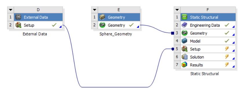
Figure 7: The ANSYS WorkBench set-up linking The ROCKY data through External Data to the model (Ensure in the ROCKY menu, that the is enabled)
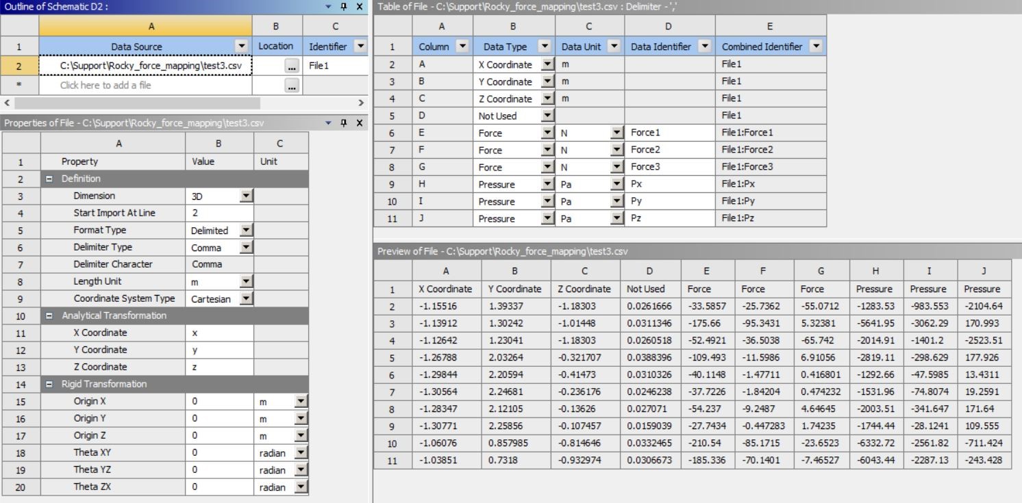
Figure 8: The ANSYS External Data set-up
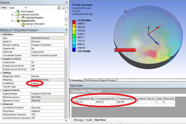
Figure 9: ANSYS Mechanical showing the imported pressure
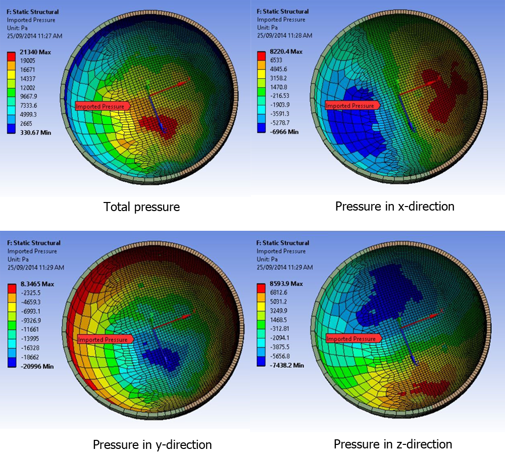
Figure 10: Contour plots of the pressure components brought in from ROCKY into ANSYS Mechanical
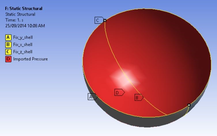

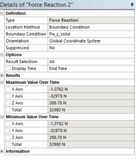
Figure 11: Model set-up and reaction forces of the ANSYS analysis for both shells (left 32,976 N) and solid shells (right 32,978 N)
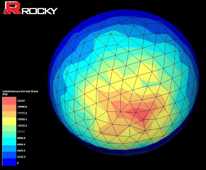
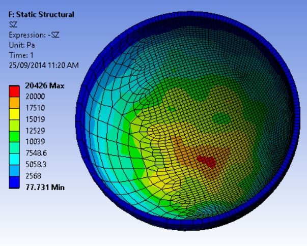
Figure 12: Comparison of the normal stress for ROCKY (left) and ANSYS (right)
This simple test model has demonstrated the new pressure mapping available with ROCKY 3.0 and the ANSYS Workbench External Data approach, outlining:
- The new version of ROCKY 3.0 outputs forces, pressures and nodal area, which enables the user to use distributed pressure components mapping to ANSYS;
- A simple External Data approach can be used to map the ROCKY pressures to ANSYS pressures;
- The ROCKY mesh can be significantly different from the ANSYS mesh;
- It is recommended to use a ROCKY mesh large enough to have particles colliding with each element, but small enough to get a reasonable gradient and accuracy in the pressure interpolation results;
Our next post (Part 2) will demonstrate these same techniques to map loads for a more realistic scenario: loads from coal particles discharging from a coal wagon. In the meantime, for more information please contact info@leapaust.com.au